New features of AbiPy v0.7

M. Giantomassi and the AbiPy group

9th international ABINIT developer workshop
20-22nd May 2019 - Louvain-la-Neuve, Belgium


Use the Space key to navigate through all slides.

What is AbiPy?

Python package for:

  • Generating ABINIT input files automatically
  • Post-processing output results (netcdf and text files)
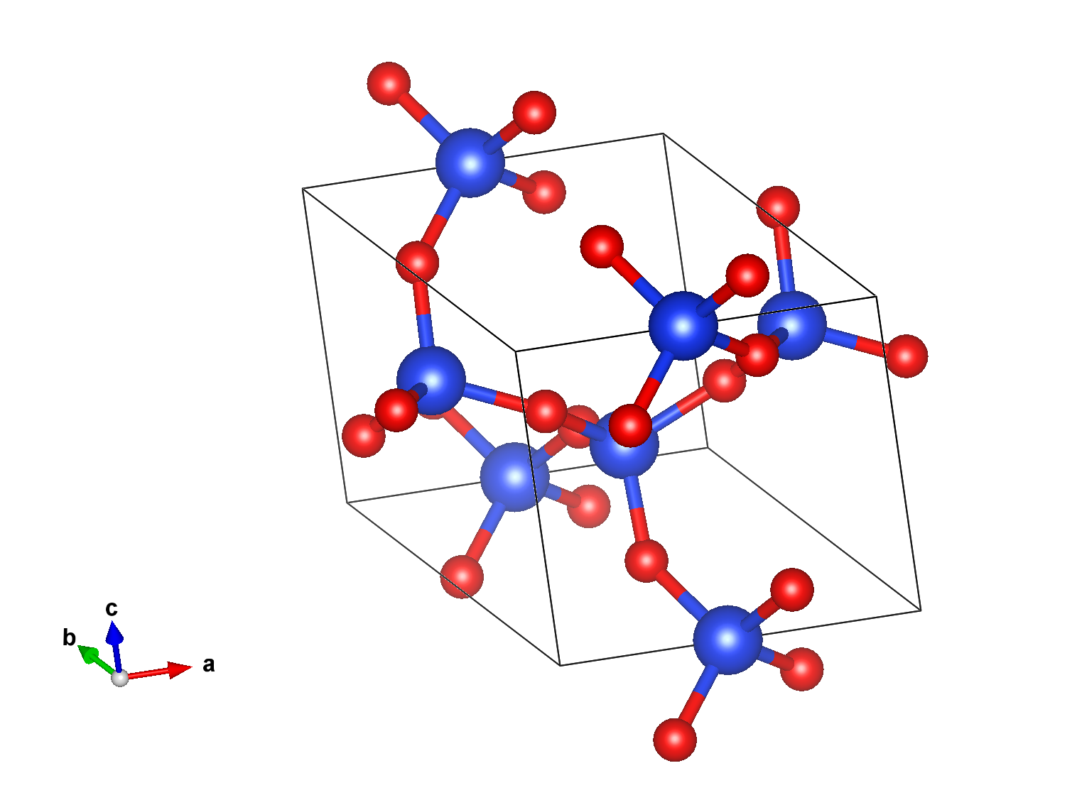
  • Interfacing ABINIT with external tools (e.g. Vesta)
  • Creating and executing workflows (band structures, DFPT, $GW$, BSE…)

Why python?

How to install AbiPy

Using pip and python wheels:

    pip install abipy --user

Using conda (recommended):

    conda install abipy --channel abinit 

From the github repository (develop mode):

    git clone https://github.com/abinit/abipy.git
    cd abipy 
    python setup.py develop


For further info see http://abinit.github.io/abipy/installation.html

AbiPy documentation with galleries of matplotlib examples and workflows

In [57]:
%embed https://abinit.github.io/abipy/index.html
Out[57]:

Jupyter notebooks with examples and lessons inspired by the official tutorials

In [58]:
%embed https://nbviewer.jupyter.org/github/abinit/abitutorials/blob/master/abitutorials/index.ipynb
Out[58]:

  • Since AbiPy is not restricted to high-throughput, we'll show how to use the terminal to analyze calculations

  • Well, a python script would be much more flexible but the goal here is to show that one can replace grep, vim, gnuplot with AbiPy

No perl scripts were harmed in the making of this notebook

Command line interface

  • abiopen.py ➝ Open output files inside ipython or print/visualize file
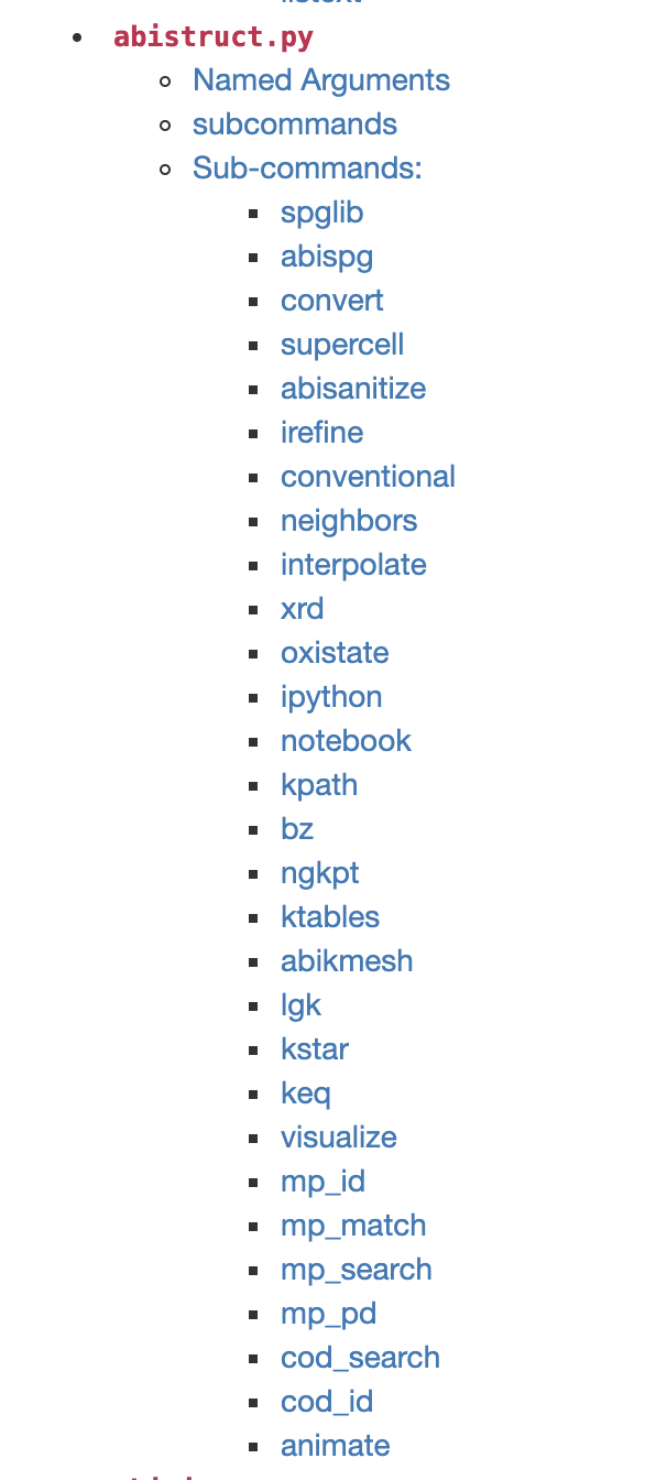
  • abistruct.py ➝ Operate on crystalline structures read from file
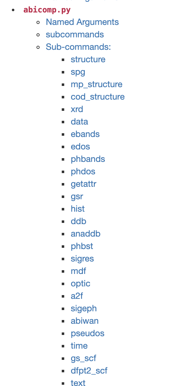
  • abicomp.py ➝ Compare multiple files (i.e. convergence studies)
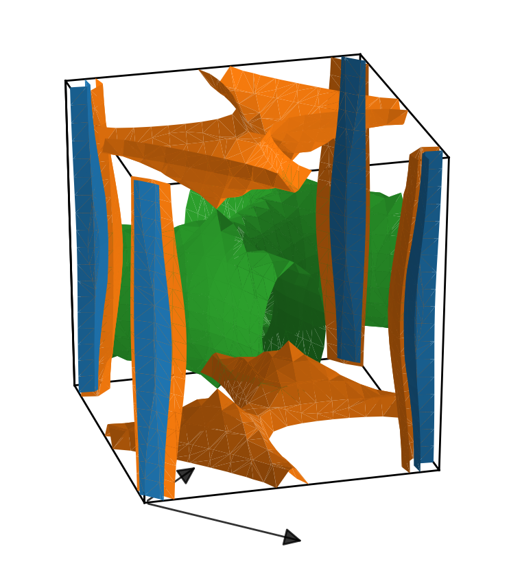
  • abiview.py ➝ Quick visualization of output files
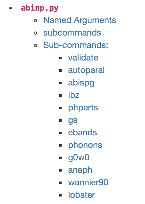
  • abinp.py ➝ Generate input files for typical calculations

Documentation

Examples

abistruct.py spglib si_scf_GSR.nc
abistruct.py convert si_scf_GSR.nc -f cif
abiopen.py si_scf_GSR.nc --print

and many more...

In [59]:
!abiopen.py si_scf_GSR.nc --print
================================= File Info =================================
Name: si_scf_GSR.nc
Directory: /Users/gmatteo/talks/abipy_intro_abidev2019
Size: 14.83 kb
Access Time: Sun May 19 20:26:25 2019
Modification Time: Sun May 12 04:20:35 2019
Change Time: Sun May 12 04:20:35 2019

================================= Structure =================================
Full Formula (Si2)
Reduced Formula: Si
abc   :   3.866975   3.866975   3.866975
angles:  60.000000  60.000000  60.000000
Sites (2)
  #  SP       a     b     c  cartesian_forces
---  ----  ----  ----  ----  -----------------------------------------------------------
  0  Si    0     0     0     [-5.89948302e-27 -1.93366148e-27  2.91016902e-27] eV ang^-1
  1  Si    0.25  0.25  0.25  [ 5.89948302e-27  1.93366148e-27 -2.91016902e-27] eV ang^-1

Abinit Spacegroup: spgid: 227, num_spatial_symmetries: 48, has_timerev: True, symmorphic: True

Stress tensor (Cartesian coordinates in GPa):

 [7.86452261e-11 5.21161758e+00 0.00000000e+00]
 [0.00000000e+00 0.00000000e+00 5.21161758e+00]]

Pressure: -5.212 (GPa)
Energy: -241.23646832 (eV)

============================== Electronic Bands ==============================
Number of electrons: 8.0, Fermi level: 5.598 (eV)
nsppol: 1, nkpt: 29, mband: 8, nspinor: 1, nspden: 1
smearing scheme: none, tsmear_eV: 0.272, occopt: 1
Direct gap:
    Energy: 2.532 (eV)
    Initial state: spin=0, kpt=[+0.000, +0.000, +0.000], weight: 0.002, band=3, eig=5.598, occ=2.000
    Final state:   spin=0, kpt=[+0.000, +0.000, +0.000], weight: 0.002, band=4, eig=8.130, occ=0.000
Fundamental gap:
    Energy: 0.562 (eV)
    Initial state: spin=0, kpt=[+0.000, +0.000, +0.000], weight: 0.002, band=3, eig=5.598, occ=2.000
    Final state:   spin=0, kpt=[+0.375, +0.375, +0.000], weight: 0.012, band=4, eig=6.161, occ=0.000
Bandwidth: 11.856 (eV)
Valence maximum located at:
    spin=0, kpt=[+0.000, +0.000, +0.000], weight: 0.002, band=3, eig=5.598, occ=2.000
Conduction minimum located at:
    spin=0, kpt=[+0.375, +0.375, +0.000], weight: 0.012, band=4, eig=6.161, occ=0.000

To produce a predefined set of matplotlib figures, use:

abiopen.py mgb2_kpath_FATBANDS.nc --expose --seaborn

abiopen_expose

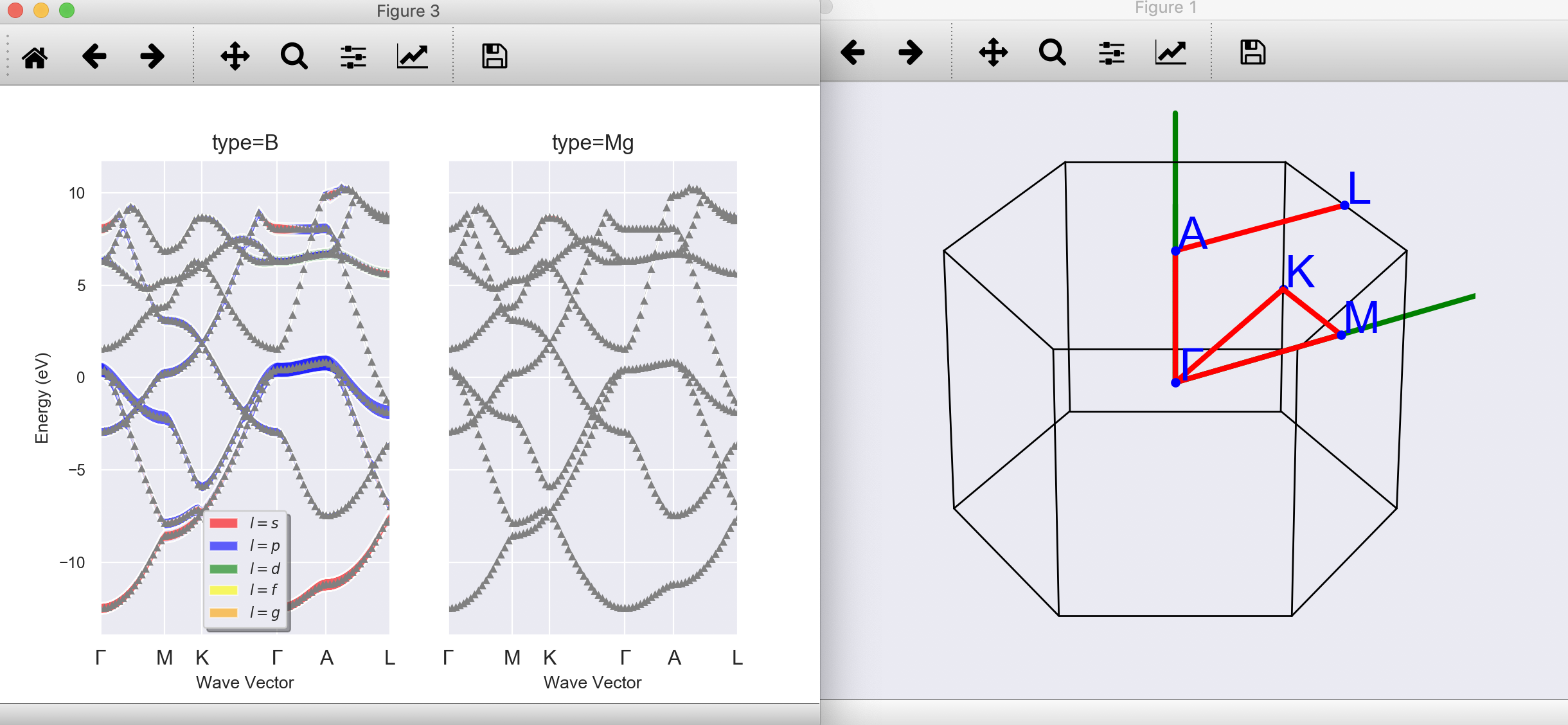
Replace --expose with --notebook to generate a jupyter notebook with predefined python code

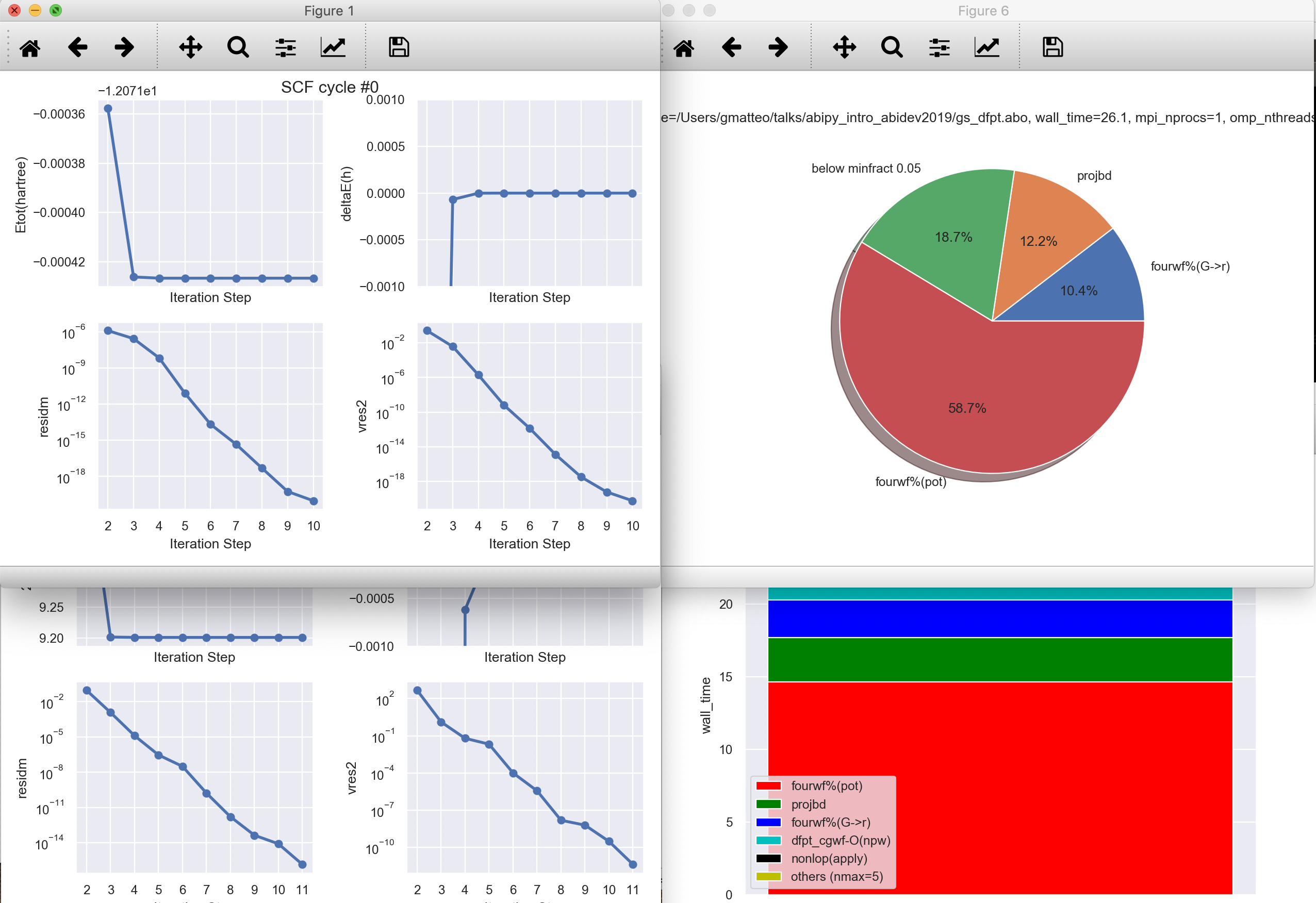
abiopen.py supports output files (note abo extension):

In [60]:
!abiopen.py gs_dfpt.abo -p 
ndtset: 3, completed: True
Full Formula (C2)
Reduced Formula: C
abc   :   2.508336   2.508336   2.508336
angles:  60.000000  60.000000  60.000000
Sites (2)
  #  SP       a     b     c
---  ----  ----  ----  ----
  0  C     0     0     0
  1  C     0.25  0.25  0.25

Abinit Spacegroup: spgid: 227, num_spatial_symmetries: 48, has_timerev: True, symmorphic: True

========================= Dimensions of calculation =========================
         intxc  ionmov  iscf  lmnmax  lnmax  mgfft  mpssoang  mqgrid  natom  \
dataset                                                                       
1            0     0.0     7       1      1     24         2    3001      2   
2            0     NaN     7       1      1     24         2    3001      2   
3            0     NaN     7       1      1     24         2    3001      2   

         nloc_mem  nspden  nspinor  nsppol  nsym  n1xccc  ntypat  occopt  \
dataset                                                                    
1               1       1        1       1    48    2501       1       1   
2               1       1        1       1    48    2501       1       1   
3               1       1        1       1    48    2501       1       1   

         xclevel  mband  mffmem  mkmem  mpw   nfft  nkpt  mem_per_proc_mb  \
dataset                                                                     
1              1      4       1      8  609  13824     8            4.791   
2              1      4       1     64  609  13824    64           11.529   
3              1      4       1     64  609  13824    64           12.285   

         wfk_size_mb  denpot_size_mb spg_symbol  spg_number  \
dataset                                                       
1              0.299           0.107      Fd-3m         227   
2              2.381           0.107      Fd-3m         227   
3              2.381           0.107      Fd-3m         227   

                                bravais  
dataset                                  
1        Bravais cF (face-center cubic)  
2        Bravais cF (face-center cubic)  
3        Bravais cF (face-center cubic)  
 

and log files as well:

In [61]:
!abiopen.py run.log -p 
Events found in /Users/gmatteo/talks/abipy_intro_abidev2019/run.log

[1] <AbinitComment at m_dtfil.F90:1082>
    Output file: run.abo already exists.
    
[2] <AbinitComment at m_dtfil.F90:1106>
    Renaming old run.abo to run.abo0001
    
[3] <AbinitWarning at m_mpinfo.F90:2295>
    nkpt*nsppol (29) is not a multiple of nproc_kpt (2)
    The k-point parallelisation is not efficient.
    
[4] <AbinitWarning at m_mpinfo.F90:2295>
    nkpt*nsppol (29) is not a multiple of nproc_kpt (2)
    The k-point parallelisation is not efficient.
    
[5] <AbinitComment at m_xgScalapack.F90:237>
    xgScalapack in auto mode
    
[6] <AbinitWarning at m_phonons.F90:3215>
    ph_nqpath <= 0 or ph_ndivsm <= 0. Phonon bands won't be produced. returning
    
[7] <AbinitComment at m_xgScalapack.F90:237>
    xgScalapack in auto mode
    
[8] <AbinitWarning at m_phonons.F90:3215>
    ph_nqpath <= 0 or ph_ndivsm <= 0. Phonon bands won't be produced. returning
    
num_errors: 0, num_warnings: 4, num_comments: 4, completed: True

If you are still using perl scripts to extract data from the main output file, check this out:

abiopen.py gs_dfpt.abo --expose --seaborn

The introduction of Yaml documents in the main output (cfr. Theo's talk) will facilitate the implementation of new post-processing tools...

It works with any file providing a structure object (.nc, .abi, .cif …)

Convert structure from netcdf format to CIF (abivars, xsf, poscar, qe, siesta, wannier90, json)

In [62]:
!abistruct.py convert si_scf_GSR.nc -f cif
# generated using pymatgen
data_Si
_symmetry_space_group_name_H-M   'P 1'
_cell_length_a   3.86697464
_cell_length_b   3.86697464
_cell_length_c   3.86697464
_cell_angle_alpha   60.00000000
_cell_angle_beta   60.00000000
_cell_angle_gamma   60.00000000
_symmetry_Int_Tables_number   1
_chemical_formula_structural   Si
_chemical_formula_sum   Si2
_cell_volume   40.88829228
_cell_formula_units_Z   2
loop_
 _symmetry_equiv_pos_site_id
 _symmetry_equiv_pos_as_xyz
  1  'x, y, z'
loop_
 _atom_site_type_symbol
 _atom_site_label
 _atom_site_symmetry_multiplicity
 _atom_site_fract_x
 _atom_site_fract_y
 _atom_site_fract_z
 _atom_site_occupancy
  Si  Si1  1  0.000000  0.000000  0.000000  1
  Si  Si2  1  0.250000  0.250000  0.250000  1

Are you still using cut3d to export the structure in a format that other applications can understand?

abistruct.py visualize run_si02.abi

Supports also ovito, xcrysden, vtk, mayavi, matplotlib (Use --application option)

Connect to the materials project database to find similar structures.

In [66]:
!abistruct.py mp_match si_scf_GSR.nc
# Found 1 structures in Materials Project database (use `verbose` to get further info)

 
########################## abivars input for mp-149 ##########################
# Full Formula (Si2)
# Reduced Formula: Si
# abc   :   3.866975   3.866975   3.866975
# angles:  60.000000  60.000000  60.000000
# 
# Spglib space group info (magnetic symmetries not taken into account).
# Spacegroup: Fd-3m (227), Hall: F 4d 2 3 -1d, Abinit spg_number: None
# Crystal_system: cubic, Lattice_type: cubic, Point_group: m-3m
# 
#   Idx  Symbol    Reduced_Coords              Wyckoff      EqIdx
# -----  --------  --------------------------  ---------  -------
#     0  Si        +0.87500 +0.87500 +0.87500  (2a)             0
#     1  Si        +0.12500 +0.12500 +0.12500  (2a)             0

 natom 2
 ntypat 1
 typat 1 1
 znucl 14
 xred
    0.8750000000    0.8750000000    0.8750000000
    0.1250000000    0.1250000000    0.1250000000
 acell    1.0    1.0    1.0
 rprim
    6.3285005334    0.0000000000    3.6537614829
    2.1095001778    5.9665675247    3.6537614829
    0.0000000000    0.0000000000    7.3075229659


To search by chemical system or formula (no FILE required)

In [67]:
!abistruct.py mp_search LiF
# Found 3 structures in Materials Project database (use `verbose` to get further info)

           pretty_formula  e_above_hull  energy_per_atom  \
mp-1185301            LiF      0.007565        -4.837577   
mp-1009009            LiF      0.273111        -4.572031   
mp-1138               LiF      0.000000        -4.845142   

            formation_energy_per_atom  nsites     volume spacegroup.symbol  \
mp-1185301                  -3.173315       4  42.223600            P6_3mc   
mp-1009009                  -2.907769       2  16.768040             Pm-3m   
mp-1138                     -3.180880       2  17.022154             Fm-3m   

            spacegroup.number  band_gap  total_magnetization material_id  \
mp-1185301                186    7.4778         0.000000e+00  mp-1185301   
mp-1009009                221    7.5593         0.000000e+00  mp-1009009   
mp-1138                   225    8.7161         9.000000e-07     mp-1138   

                   a         b         c  alpha  beta       gamma  
mp-1185301  3.139544  3.139544  4.946425   90.0  90.0  120.000008  
mp-1009009  2.559533  2.559533  2.559533   90.0  90.0   90.000000  
mp-1138     2.887419  2.887419  2.887419   60.0  60.0   60.000000  
 
 
######################## abivars input for mp-1185301 ########################
# Full Formula (Li2 F2)
# Reduced Formula: LiF
# abc   :   3.139544   3.139544   4.946425
# angles:  90.000000  90.000000 120.000008
# 
# Spglib space group info (magnetic symmetries not taken into account).
# Spacegroup: P6_3mc (186), Hall: P 6c -2c, Abinit spg_number: None
# Crystal_system: hexagonal, Lattice_type: hexagonal, Point_group: 6mm
# 
#   Idx  Symbol    Reduced_Coords              Wyckoff      EqIdx
# -----  --------  --------------------------  ---------  -------
#     0  Li        +0.00000 +0.00000 +0.38019  (2b)             0
#     1  Li        +0.33333 +0.66667 +0.88019  (2b)             0
#     2  F         +0.00000 +0.00000 +0.99481  (2b)             2
#     3  F         +0.33333 +0.66667 +0.49481  (2b)             2

 natom 4
 ntypat 2
 typat
 1 1 2
 2
 znucl 3 9
 xred
    0.0000000000    0.0000000000    0.3801910000
    0.3333333333    0.6666666667    0.8801900000
    0.0000000000    0.0000000000    0.9948070000
    0.3333333333    0.6666666667    0.4948100000
 acell    1.0    1.0    1.0
 rprim
    5.9328791503    0.0000000000    0.0000000000
   -2.9664403365    5.1380236222    0.0000000000
    0.0000000000    0.0000000000    9.3473877186


######################## abivars input for mp-1009009 ########################
# Full Formula (Li1 F1)
# Reduced Formula: LiF
# abc   :   2.559533   2.559533   2.559533
# angles:  90.000000  90.000000  90.000000
# 
# Spglib space group info (magnetic symmetries not taken into account).
# Spacegroup: Pm-3m (221), Hall: -P 4 2 3, Abinit spg_number: None
# Crystal_system: cubic, Lattice_type: cubic, Point_group: m-3m
# 
#   Idx  Symbol    Reduced_Coords              Wyckoff      EqIdx
# -----  --------  --------------------------  ---------  -------
#     0  Li        +0.00000 +0.00000 +0.00000  (1a)             0
#     1  F         +0.50000 +0.50000 +0.50000  (1b)             1

 natom 2
 ntypat 2
 typat 1 2
 znucl 3 9
 xred
    0.0000000000    0.0000000000    0.0000000000
    0.5000000000    0.5000000000    0.5000000000
 acell    1.0    1.0    1.0
 rprim
    4.8368167948    0.0000000000    0.0000000000
    0.0000000000    4.8368167948    0.0000000000
    0.0000000000    0.0000000000    4.8368167948


######################### abivars input for mp-1138 #########################
# Full Formula (Li1 F1)
# Reduced Formula: LiF
# abc   :   2.887419   2.887419   2.887419
# angles:  60.000000  60.000000  60.000000
# 
# Spglib space group info (magnetic symmetries not taken into account).
# Spacegroup: Fm-3m (225), Hall: -F 4 2 3, Abinit spg_number: None
# Crystal_system: cubic, Lattice_type: cubic, Point_group: m-3m
# 
#   Idx  Symbol    Reduced_Coords              Wyckoff      EqIdx
# -----  --------  --------------------------  ---------  -------
#     0  Li        +0.00000 +0.00000 +0.00000  (1a)             0
#     1  F         +0.50000 +0.50000 +0.50000  (1b)             1

 natom 2
 ntypat 2
 typat 1 2
 znucl 3 9
 xred
    0.0000000000    0.0000000000    0.0000000000
    0.5000000000    0.5000000000    0.5000000000
 acell    1.0    1.0    1.0
 rprim
    4.7254082787    0.0000000000    2.7282157318
    1.5751360851    4.4551576322    2.7282157281
    0.0000000000    0.0000000000    5.4564314785


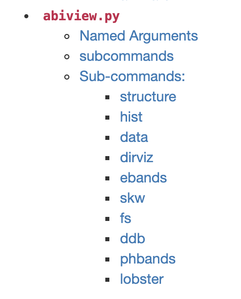
Need to call anaddb to compute and visualize ph-bands and DOS from DDB?

abiview.py ddb ZnSe_hex_qpt_DDB --seaborn

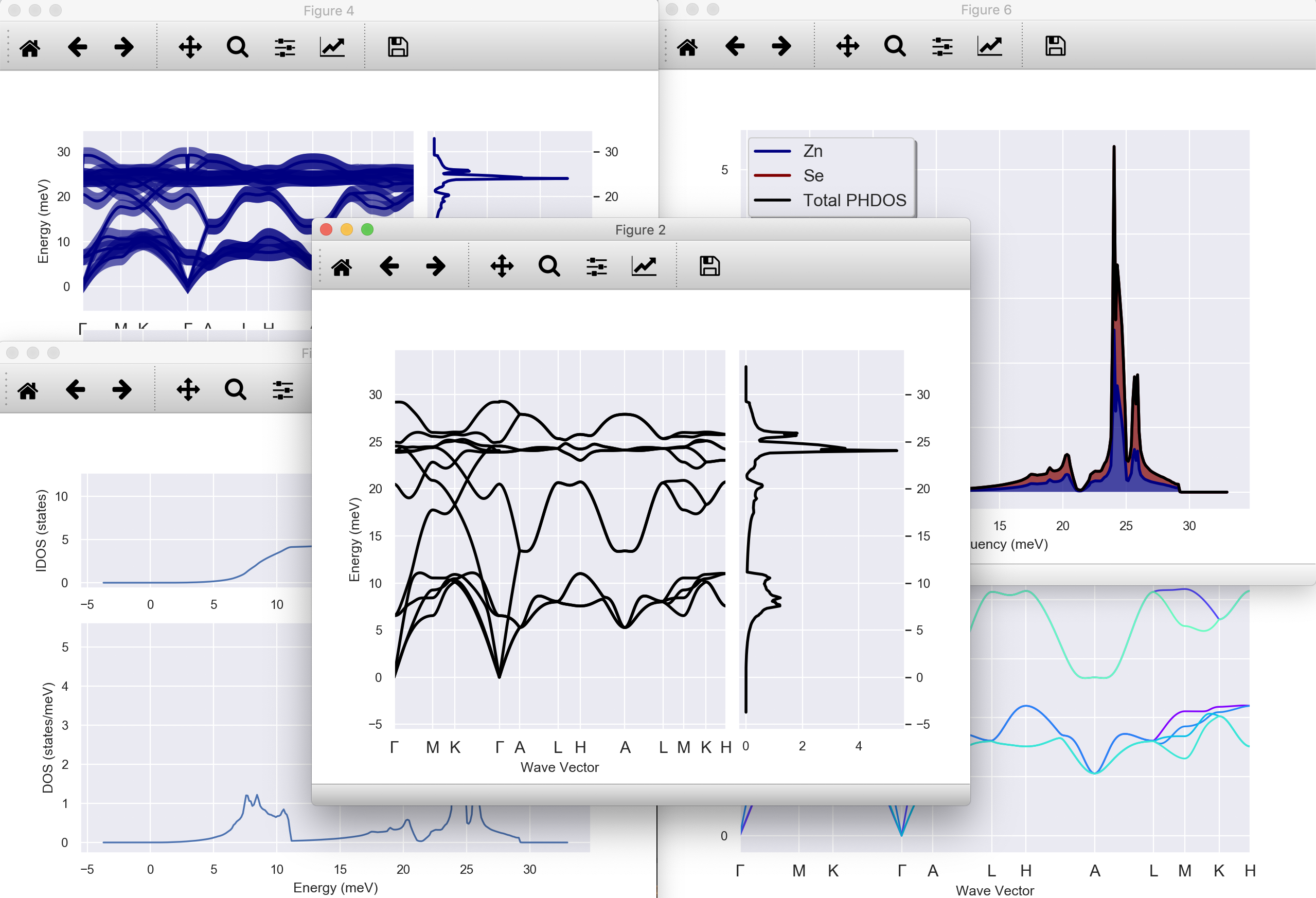
Add --phononwebsite to visualize data on the phononwebsite by Henrique

Need to get a quick look at the Fermi surface?

abiview.py fs mgb2_kmesh181818_FATBANDS.nc

Use -a xsf for Xcrysden or -a mayavi for Mayavi backend

To compare multiple structures:

In [68]:
!abicomp.py structure *.cif si_nscf_GSR.nc `find . -name *_DDB`
Spglib options: symprec= 0.001 angle_tolerance= 5.0
Lattice parameters:
                  formula  natom  alpha  beta  gamma         a         b  \
AlAs.cif          Al1 As1      2   60.0  60.0   60.0  3.970101  3.970101   
si.cif                Si2      2   60.0  60.0   60.0  3.866975  3.866975   
si_nscf_GSR.nc        Si2      2   60.0  60.0   60.0  3.866975  3.866975   
ZnSe_hex_qpt_DDB  Zn2 Se2      4   90.0  90.0  120.0  4.050187  4.050187   

                         c     volume abispg_num spglib_symb  spglib_num  \
AlAs.cif          3.970101  44.247584       None       F-43m         216   
si.cif            3.866975  40.888292       None       Fd-3m         227   
si_nscf_GSR.nc    3.866975  40.888292        227       Fd-3m         227   
ZnSe_hex_qpt_DDB  6.652328  94.504936          0      P6_3mc         186   

                 spglib_lattice_type  
AlAs.cif                       cubic  
si.cif                         cubic  
si_nscf_GSR.nc                 cubic  
ZnSe_hex_qpt_DDB           hexagonal  
 

Note shell wildcard characters and Unix find inside backticks (bash rocks!)

Using ElectronBandsPlotter to visualize multiple band structures:

abicomp.py ebands *_GSR.nc

Bash is handy but python is more flexible

Let's use the DdbRobot to compare phonons obtained with different ${\bf k}$-meshes and smearing values:
In [70]:
paths = [
    "mgb2_888k_0.01tsmear_DDB",
    "mgb2_888k_0.04tsmear_DDB",
    "mgb2_121212k_0.01tsmear_DDB",
    "mgb2_121212k_0.04tsmear_DDB",
]

paths = [os.path.join(abidata.dirpath, "refs", "mgb2_phonons_nkpt_tsmear", f) 
         for f in paths]

robot = abilab.DdbRobot()
for i, path in enumerate(paths):
    robot.add_file(path, path)
In [71]:
# Define function to change labels:
func = lambda ddb: "nkpt: %s, tsmear: %.2f" % (
    ddb.header["nkpt"], ddb.header["tsmear"])

robot.remap_labels(func)
robot
Out[71]:
  1. nkpt: 256, tsmear: 0.01
  2. nkpt: 256, tsmear: 0.04
  3. nkpt: 864, tsmear: 0.01
  4. nkpt: 864, tsmear: 0.04

Now we can build a dataframe with the most important parameters:

In [72]:
robot.get_params_dataframe()
Out[72]:
nkpt nsppol ecut tsmear occopt ixc nband usepaw
nkpt: 256, tsmear: 0.01 256 1 35.0 0.01 4 1 8 0
nkpt: 256, tsmear: 0.04 256 1 35.0 0.04 4 1 8 0
nkpt: 864, tsmear: 0.01 864 1 35.0 0.01 4 1 8 0
nkpt: 864, tsmear: 0.04 864 1 35.0 0.04 4 1 8 0

and check that all DDBs have been computed with the same crystalline structure:

In [73]:
robot.get_lattice_dataframe()
Out[73]:
formula natom alpha beta gamma a b c volume abispg_num spglib_symb spglib_num spglib_lattice_type
nkpt: 256, tsmear: 0.01 Mg1 B2 3 90.0 90.0 120.0 3.086 3.086 3.523 29.055953 0 P6/mmm 191 hexagonal
nkpt: 256, tsmear: 0.04 Mg1 B2 3 90.0 90.0 120.0 3.086 3.086 3.523 29.055953 0 P6/mmm 191 hexagonal
nkpt: 864, tsmear: 0.01 Mg1 B2 3 90.0 90.0 120.0 3.086 3.086 3.523 29.055953 0 P6/mmm 191 hexagonal
nkpt: 864, tsmear: 0.04 Mg1 B2 3 90.0 90.0 120.0 3.086 3.086 3.523 29.055953 0 P6/mmm 191 hexagonal

To analyze the effect of k-sampling/smearing on the vibrational properties:

In [74]:
# Invoke anaddb and store results
r = robot.anaget_phonon_plotters(nqsmall=2)

r.phbands_plotter.gridplot_with_hue("tsmear", with_dos=True);

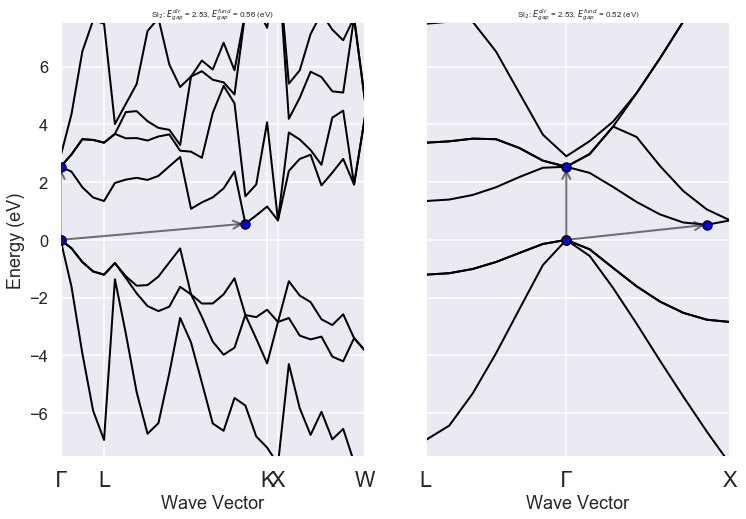
Input file for band structure calculation + DOS

  1. GS run to get the density
  2. NSCF run along high-symmetry k-path
  3. NSCF run with k-mesh to compute the DOS
In [77]:
multi = abilab.ebands_input(structure="si.cif", 
                            pseudos="14si.pspnc",
                            ecut=8, 
                            spin_mode="unpolarized", 
                            smearing=None, 
                            dos_kppa=5000)

multi.get_vars_dataframe("kptopt", "iscf", "ngkpt")
Out[77]:
kptopt iscf ngkpt
dataset 0 1 None [8, 8, 8]
dataset 1 -11 -2 None
dataset 2 1 -2 [14, 14, 14]

To build an input for SCF+NSCF run with (relaxed) structure from the materials project database:

    abinp.py ebands mp-149          

abinp.py is handy for generating input files quickly but it cannot compete with the flexibility of the python interface:

In [79]:
def make_scf_input(ecut=2, ngkpt=(4, 4, 4)):
    """
    Generate an `AbinitInput` to perform GS calculation for AlAs.

    Args:
        ecut: Cutoff energy in Ha.
        ngkpt: k-mesh divisions

    Return:
        `AbinitInput` object
    """
    gs_inp = abilab.AbinitInput(structure="AlAs.cif",
                                pseudos=["13al.pspnc", "33as.pspnc"])

    # Set the value of the Abinit variables needed for GS runs.
    gs_inp.set_vars(
        nband=4,
        ecut=ecut,
        ngkpt=ngkpt,
        nshiftk=4,
        shiftk=[0.0, 0.0, 0.5,   # This gives the usual fcc Monkhorst-Pack grid
                0.0, 0.5, 0.0,
                0.5, 0.0, 0.0,
                0.5, 0.5, 0.5],
        tolvrs=1.0e-10,
    )

    return gs_inp
In [80]:
make_scf_input()
Out[80]:
############################################################################################
# SECTION: basic
############################################################################################
nband 4
ecut 2
ngkpt 4 4 4
nshiftk 4
shiftk
0.0 0.0 0.5
0.0 0.5 0.0
0.5 0.0 0.0
0.5 0.5 0.5
tolvrs 1e-10
############################################################################################
# STRUCTURE
############################################################################################
natom 2
ntypat 2
typat 1 2
znucl 13 33
xred
0.0000000000 0.0000000000 0.0000000000
0.2500000000 0.2500000000 0.2500000000
acell 1.0 1.0 1.0
rprim
6.4972715500 0.0000000000 3.7512014784
2.1657571833 6.1256863630 3.7512014784
0.0000000000 0.0000000000 7.5024029568

Moreover, from an AbiniInput one can easily build more complicate workflows:

In [81]:
def build_flow_alas_phonons():
    """
    Build and return a Flow to compute the dynamical matrix on a (2, 2, 2) qmesh
    as well as DDK and Born effective charges.
    The final DDB with all perturbations will be merged automatically and placed
    in the Flow `outdir` directory.
    """
    from abipy import flowtk
    scf_input = make_scf_input(ecut=6, ngkpt=(4, 4, 4))
    return flowtk.PhononFlow.from_scf_input("flow_alas_phonons", scf_input,
                                            ph_ngqpt=(2, 2, 2), with_becs=True)
Abipy will call Abinit to get the list of DFPT perturbations and…
In [82]:
flow_phbands = build_flow_alas_phonons()
flow_phbands.get_graphviz()
Out[82]:
flow PhononFlow, node_id=1218, workdir=flow_alas_phonons clusterw0 Work (w0) clusterw1 BecWork (w1) clusterw2 PhononWork (w2) clusterw3 PhononWork (w3) w0_t0 w0_t0 ScfTask w1_t0 w1_t0 DdkTask w0_t0->w1_t0 WFK w1_t1 w1_t1 DdkTask w0_t0->w1_t1 WFK w1_t2 w1_t2 DdkTask w0_t0->w1_t2 WFK w1_t3 w1_t3 BecTask w0_t0->w1_t3 WFK w1_t4 w1_t4 BecTask w0_t0->w1_t4 WFK w2_t0 w2_t0 PhononTask w0_t0->w2_t0 WFK w2_t1 w2_t1 PhononTask w0_t0->w2_t1 WFK w2_t2 w2_t2 PhononTask w0_t0->w2_t2 WFK w2_t3 w2_t3 PhononTask w0_t0->w2_t3 WFK w3_t0 w3_t0 PhononTask w0_t0->w3_t0 WFK w3_t1 w3_t1 PhononTask w0_t0->w3_t1 WFK w1_t0->w1_t3 DDK w1_t0->w1_t4 DDK w1_t1->w1_t3 DDK w1_t1->w1_t4 DDK w1_t2->w1_t3 DDK w1_t2->w1_t4 DDK

Future developments

Post-processing tools

  • Support for more netcdf files
  • More post-processing tools for MD calculations
  • More converters and interfaces for third-party applications
  • Integrate AbiPy with jupyterlab to create a flexible graphical enviroment for Abinit exposing (part) of the python API
  • Explore web-based technologies for data analysis and visualization (plotly, dash)
  • Develop toolkit to build web apps powered by AbiPy and pymatgen to disseminate scientific results.

Continuous Integration

  • Use AbiPy programmatic interface to implement:

    • Validation of parallel algorithms for np in range(1, N)
    • Stress testing
    • Benchmarks