Automating ABINIT calculations with AbiPy
M. Giantomassi and the AbiPy group
Boston MA, 3 March 2019
These slides have been generated using jupyter, nbconvert and revealjs
The notebook can be downloaded from this github repo
To install and configure the software, follow these installation instructions
![]()
What is AbiPy?
Python package for:
- Generating ABINIT input files automatically
- Post-processing output results (netcdf and text files)
- Interfacing ABINIT with external tools (e.g. Vesta)
- Creating and executing workflows (band structures, phonons, $GW$…)
Project:
- Developed and maintained by the ABINIT community
- Used by developers to validate, profile and optimize ABINIT
- Hosted on github
- Release under the GPLv2 license
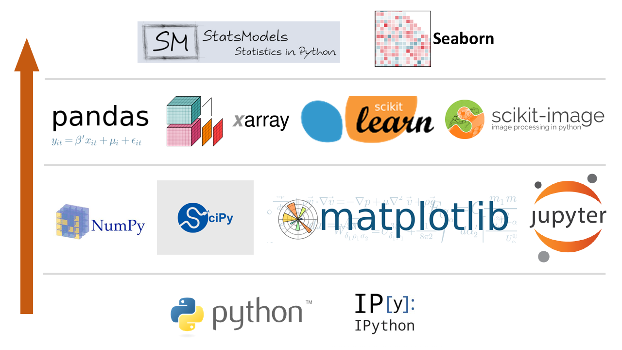
Why python?
- Easy to use and to learn
- Great support for science (numpy, scipy, pandas, matplotlib …)
- Interactive environments (ipython, jupyter notebooks, GUIs)
- More powerful and flexible than Fortran for implementing the high-level logic needed in modern ab-initio workflows
- pymatgen ecosystem and the materials project database…
AbiPy design principles
- Extend the pymatgen code-base with ABINIT-specific objects
Layered structure designed for different use-cases:
Closely connected to the ABINIT executable:
- CPU-intensive algorithms performed by ABINIT (Fortran + MPI + OpenMP)
- Glue code implemented in python
ABINIT and AbiPy communicate through netcdf files
- Portable binary format implemented in C
- Fortran/Python bindings and support for parallel MPI-IO (HDF5)
- ETSF-IO specifications for crystalline structures, wavefunctions, densities…
How to install AbiPy
Using pip and python wheels:
pip install abipy --user
Using conda (recommended):
conda install abipy --channel abinit
From the github repository (develop mode):
    git clone https://github.com/abinit/abipy.git
    cd abipy
    python setup.py develop
For further info see http://abinit.github.io/abipy/installation.html
AbiPy documentation
%embed https://abinit.github.io/abipy/index.html
Jupyter notebooks with examples and lessons
%embed https://nbviewer.jupyter.org/github/abinit/abitutorials/blob/master/abitutorials/index.ipynb
What do we need to automate calculations?
- Tools to parse and analyze output results
- python API to generate input files
High-level logic for:
- Managing complicated workflows
- Exposing task parallelism (independent steps can be executed in parallel)
- Handling runtime errors and restarting calculations
- Saving final results in machine-readable format (e.g. databases)
Let's discuss the different parts step by step…
AbiPy post-processing tools
Main entry point:
from abipy import abilab
abifile = abilab.abiopen("filename.nc")
where filename.nc is a netcdf file (support also text files e.g. run.abo, run.log, out_DDB)
abifile is the AbiFile subclass associated to the given file extension:
- GSR.nc ➝ GsrFile
- HIST.nc ➝ HistFile
- More than 45 file extensions supported (see
abiopen.py --help)
Command line interface: use
abiopen.py FILEto:- open the file inside the ipython terminal
- print info to terminal (
--printoption) - produce a predefined set of matplotlib figures (
--exposeoption) - generate jupyter notebooks (
--notebookoption)
Before we start, we need to import two AbiPy modules:
from abipy import abilab
import abipy.data as abidata
Now we can open our netcdf file with abiopen
gsr_kpath = abilab.abiopen("si_nscf_GSR.nc")
This function returns an AbiFile object provinding access to physical properties.
Conventions:
- abifile.structure ➝ crystalline structure (subclass of pymatgen Structure)
- abifile.ebands ➝ electron band energies
- abifile.ebands.kpoints ➝ list of k-points (k-path, IBZ)
- abifile.phbands ➝ phonon frequencies and displacements
Several AbiPy objects provide plot methods returning matplotlib figures
The GsrFile has a pymatgen structure:
print(gsr_kpath.structure)
Band energies, occupation factors, k-points are stored in the ebands object
print(gsr_kpath.ebands)
The ebands object has a list of k-points that can be visualized with:
gsr_kpath.ebands.kpoints.plot();

To plot the band structure, use:
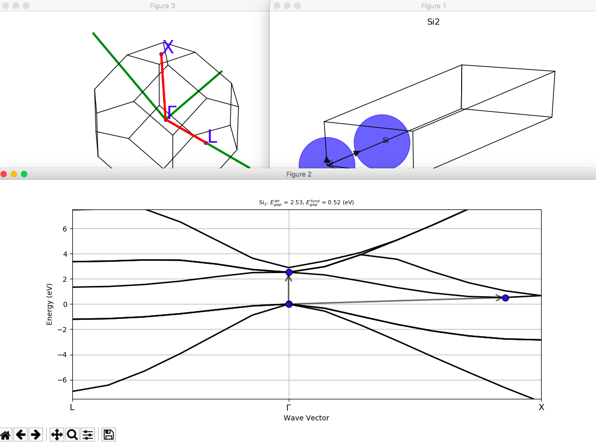
gsr_kpath.ebands.plot(with_gaps=True, title="Silicon band structure");

Band energies can be given either along a k-path or in the irreducible Brillouin zone (IBZ):
with abilab.abiopen("si_scf_GSR.nc") as scf_gsr:
    ebands_kmesh = scf_gsr.ebands
    print(ebands_kmesh.kpoints)
To compute the density of states (DOS), we need energies in the IBZ:
edos = ebands_kmesh.get_edos()
edos.plot();

Plotting bands with DOS is easy:
gsr_kpath.ebands.plot_with_edos(edos);

Use ElectronBandsPlotter to visualize multiple band structures:
plotter = abilab.ElectronBandsPlotter()
plotter.add_ebands(label="BZ sampling", bands="si_scf_GSR.nc")
plotter.add_ebands(label="k-path", bands="si_nscf_GSR.nc")
plotter.gridplot(with_gaps=True);

Other files supported by AbiPy
- GSR.nc ➝ Ground-state results produced by SCF/NSCF runs
- HIST.nc ➝ Structural relaxation and molecular dynamics
- FATBANDS.nc ➝ Fatbands and LM-projected DOS for electrons
- DDB: ➝ dynamical matrix, Born effective charges, elastic constants…
- SIGRES.nc ➝ $GW$ calculations ($\Sigma^{e-e}$ self-energy)
- MDF.nc ➝ Bethe-Salpeter calculations
- ABIWAN.nc ➝ netcdf file produced by Abinit with wannier90 results
- SIGEPH.nc ➝ electron-phonon self-energy ($\Sigma^{e-ph}$)
- …
Jupter notebooks with examples available here
Abipy Robots
High-level interface to operate on multiple files with the same file extension
Useful for:
- convergence studies
- producing multiple plots
- building Pandas dataframes (data in tabular format powered by python)
Each Robot is associated to a file extension, e.g.
- GSR.nc ➝ GsrRobot
- DDB ➝ DdbRobot
Robots can be constructed from:
- List of filenames
- Directories and regular expressions
Command line interface provided by the abicomp.py script:
To generate notebook to compare multiple GSR files, use:
abicomp.py gsr out1_GSR.nc out2_GSR.nc --notebook
ls flow_base3_ngkpt
Let's construct a GsrRobot with:
robot_enekpt = abilab.GsrRobot.from_dir("flow_base3_ngkpt");
Files can be accessed with list-like or dict-like syntax:
robot_enekpt.abifiles[0]
robot_enekpt["out0_GSR.nc"]
Now we can use the robot methods to build pandas DataFrames:
ene_table = robot_enekpt.get_dataframe()
print(ene_table.keys())
Jupyter knows how to visualize DataFrames:
ene_table
Dataframes are great as we can use python to operate on the data:
ene_table.sort_values(by="nkpt", inplace=True)

# Add 2 columns with energies in Ha and difference wrt to the last point.
ene_table["energy_Ha"] = ene_table["energy"] * abilab.units.eV_to_Ha
ene_table["ediff_Ha"] = ene_table["energy_Ha"] - ene_table["energy_Ha"][-1]

# Select columns with the syntax:
ene_table[["nkpt", "energy", "energy_Ha", "ediff_Ha"]]
- Dataframes can be exported to different formats: CSV, $Latex$, JSON, Excel, ...
- High-level plotting interface provided by seaborn
- Explore your DataFrames inside jupyter with qgrid
- Use ene_table.to_clipboard() to copy to clipboard and paste into spreadsheet editor
We can also use the pandas built-in API to plot the data with matplotlib:
ene_table.plot(x="nkpt", y=["energy_Ha", "ediff_Ha", "pressure"],
               style="-o", subplots=True);

Command line interface provided by the abicomp.py script
See also lesson_base3
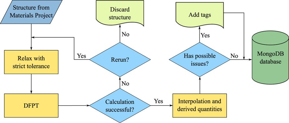
Post-processing the DFPT results available in the MP database
- More than 1500 DFPT calculations done with abiflows (Petretto et al.)
- Results available on the materials project website (including the DDB files)
Let's assume we want to reuse the raw data for our research work:
- Handling 1500 tabs in the web browser is not feasible
- We need a programmatic interface to automate stuff.
With python we can easily connect the different parts of the puzzle:
- REST API to get the raw data (DDB) from the MP database
- Computation of phonons, thermodinamical properties, Born effective charges, dielectric tensor, IR spectrum with ABINIT
- Post-processing with AbiPy
For a more comprehensive discussion see this abitutorial
To download a DDB file from the materials project database:
ddb = abilab.DdbFile.from_mpid("mp-1009129")
print(ddb)
Once we have a DdbFile object, we can call anaddb to compute phonon bands and DOS:
# Return PHBST and PHDOS netcdf files.
phbstnc, phdosnc = ddb.anaget_phbst_and_phdos_files(
    ndivsm=20, nqsmall=20, lo_to_splitting=True, asr=2,
    chneut=1, dipdip=1, dos_method="tetra")
and extract the phonon bands and the phonon DOS objects with:
phbands = phbstnc.phbands
phdos = phdosnc.phdos
print(phbands)
To plot the phonon band structure including LO-TO splitting:
phbands.plot(title="MgO phonons with LO-TO splitting");

We can also plot the phonon bands and the DOS on the same figure with:
phbands.plot_with_phdos(phdos, units="Thz", title="AlAs phonons bands and DOS");

Thermodynamic properties as function of temperature T:
phdos.plot_harmonic_thermo();

How to automate input file generation with AbiPy

AbinitInput object
Programmatic interface to generate input files:
- Dict-like object storing ABINIT variables
- Methods to set multiple variables (e.g. k-path from structure)
- Factory functions to generate input files with minimal effort
Can invoke ABINIT to get important parameters such as:
- list of k-points in the IBZ
- list of irreducible DFPT perturbations
- list of possible configurations for MPI jobs (npkpt, npfft, npband …)
To build an input, we need a structure and a list of pseudos:
inp = abilab.AbinitInput(structure="si.cif", pseudos="14si.pspnc")
Low-level API (should look familiar to Abinit users):
inp["ecut"] = 8
"ecut" in inp
Use set_vars to set the value of several variables with a single call:
inp.set_vars(kptopt=1, ngkpt=[2, 2, 2],
             shiftk=[0.0, 0.0, 0.0, 0.5, 0.5, 0.5]  # 2 shifts in one list
            );
althought it's much easier to use:
inp.set_autokmesh(nksmall=2)
An AbinitInput has a structure object
print(inp.structure.formula)
and a list of pseudopotentials
for pseudo in inp.pseudos:
    print(pseudo)
Pseudos from the PseudoDojo project provide hints for the cutoff energy.
from pseudo_dojo.core.pseudos import OfficialDojoTable
pseudo_table = OfficialDojoTable.from_dojodir('ONCVPSP-PBEsol-PDv0.4','standard')
Inside the notebook, one gets the HTML representation with links to the documentation:
inp
To generate a high-symmetry k-path (taken from an internal database)
inp.set_kpath(ndivsm=10)
- Ten points to sample the smallest segment of the k-path
- Other segments are sampled so that proportions are preserved
Interfacing Abinit with Python via AbinitInput
Once we have an AbinitInput, it is possible to execute Abinit to:
- get useful information from the Fortran code (e.g. IBZ, space group…)
- validate the input file before running the calculation
Methods invoking Abinit start with the abi prefix followed by a verb:
- inp.abiget_irred_phperts(...)
- inp.abivalidate()
Important:
To call Abinit from AbiPy, one has to prepare a configuration file (manager.yml) providing all the information required to execute/submit Abinit jobs:
$PATH,$LD_LIBRARY_PATH- modules
- python environment
- For futher info consult the documentation
Example of manager.yml for laptops (shell adapter)
qadapters:
  # List of qadapters objects
  - priority: 1
    queue:
      qtype: shell
      qname: localhost
    job:
       mpi_runner: mpirun
       pre_run:
           # abinit exec must be in $PATH
           - export PATH=$HOME/git_repos/abinit/_build/src/98_main:$PATH
    limits:
       timelimit: 30:00
       max_cores: 2
    hardware:
       num_nodes: 2
       sockets_per_node: 1
       cores_per_socket: 2
       mem_per_node: 4Gb
Examples of configuration files for clusters are available here
Use abirun.py doc_manager to get documentation inside the shell
To get the list of possible parallel configurations for this input up to max_ncpus:
inp["paral_kgb"] = 1
pconfs = inp.abiget_autoparal_pconfs(max_ncpus=5)
print("Best efficiency:\n", pconfs.sort_by_efficiency()[0])
print("Best speedup:\n", pconfs.sort_by_speedup()[0])
To get the list of irreducible phonon perturbations for a given q-point:
inp.abiget_irred_phperts(qpt=(0.25, 0, 0))
To get the irreducible perturbations for strain calculations:
inp.abiget_irred_strainperts()
- DFPT perturbations are independent hence jobs can be executed in parallel
- These methods represent the building block to generate workflows at runtime.
multi = abilab.MultiDataset(structure="si.cif", pseudos="14si.pspnc", ndtset=2)

multi.set_vars(ecut=4);
Iterating over multi gives AbinitInput objects:
all(inp["ecut"] == 4 for inp in multi)
To set the variables of a particular dataset, use:
multi[0].set_vars(ngkpt=[2, 2, 2], tsmear=0.004)
multi[1].set_vars(ngkpt=[4, 4, 4], tsmear=0.008);
To get a dataframe with the values of the variables, use:
multi.get_vars_dataframe("ngkpt", "tsmear")
The function split_datasets returns the list of AbinitInput stored in MultiDataset
gs1, gs2 = multi.split_datasets()
Factory functions for typical calculations
- Functions returning AbinitInput or MultiDataset depending on the calculation type
Minimal input from user:
- structure object or file providing it
- list of pseudos
- metavariables e.g. kppra for the BZ sampling
Default values designed to cover the most common scenarios
- Less flexible than the low-level API but easier to use
- Optional arguments to change the default behaviour (smearing="gaussian:0.1 eV")
- For a command line interface, use the abinp.py script.
To build an input for SCF+NSCF run with (relaxed) structure from the materials project database:
abinp.py ebands mp-149
Some examples...
Input file for band structure calculation + DOS
- GS run to get the density
- NSCF run along high-symmetry k-path
- NSCF run with k-mesh to compute the DOS
multi = abilab.ebands_input(structure="si.cif",
                            pseudos="14si.pspnc",
                            ecut=8,
                            spin_mode="unpolarized",
                            smearing=None,
                            dos_kppa=5000)

multi.get_vars_dataframe("kptopt", "iscf", "ngkpt")
$GW$ calculations with the plasmon-pole model. The calculation consists of:
- GS run to compute the density
- nscf-run to produce a WFK file with nscf_nband states
- Input files to compute the screening ($W$) and the self-energy ($\Sigma^{e-e} = GW$)
multi = abilab.g0w0_with_ppmodel_inputs(
    structure="si.cif", pseudos="14si.pspnc",
    kppa=1000, nscf_nband=50, ecuteps=2, ecutsigx=4, ecut=8,
    spin_mode="unpolarized")

multi.get_vars_dataframe("optdriver", "ngkpt", "nband", "ecuteps", "ecutsigx")
- nscf_nband ➝ number of bands in $GW$ (occ + empty)
- ecuteps ➝ planewave cutoff for $W_{G, G'}$ in Hartree
- ecutsigx ➝ cutoff energy for the exchange part $\Sigma_x$
- kppa ➝ k-point sampling (#kpts per reciprocal atom)
Command line interface
- abistruct.py ➝ Operate on crystalline structures read from file
- abiopen.py ➝ Open output files inside Ipython session
- abicomp.py ➝ Compare multiple files (convergence studies)
- abiview.py ➝ Quick visualization of output files
- abinp.py ➝ Generate input files for typical calculations
Use e.g.
abistruct.py --helpfor manpageabistruct.py COMMAND --helpfor help aboutCOMMAND
HTML documentation available at http://abinit.github.io/abipy/scripts/index.html
Examples
abistruct.py spglib si_scf_GSR.nc
abistruct.py convert si_scf_GSR.nc -f cif
abiopen.py si_scf_GSR.nc --print
Workflow infrastructure
Two different approaches:
AbiPy workflows:
- Lightweight implementation (pymatgen + AbiPy)
- No database required. Object persistence provided by pickle
- Ideal tool for prototyping
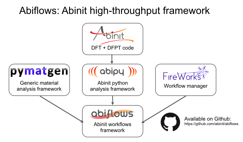
AbiFlows workflows:
- Requires MongoDb database
- Based on fireworks
- Designed and optimized for high-throughput applications
Both approaches share the same codebase (AbinitInput, factory functions, AbiPy objects).
Number and type of calculations are important ➝ choose the approach that suits to your needs.
Main features
- Support for different resource managers (Slurm, PBS, Torque, SGE, LoadLever, shell)
- autoparal: the number of MPI processes is optimized at runtime
- Error handlers for common runtime failures
- Iterative algorithms are automatically restarted by the framework
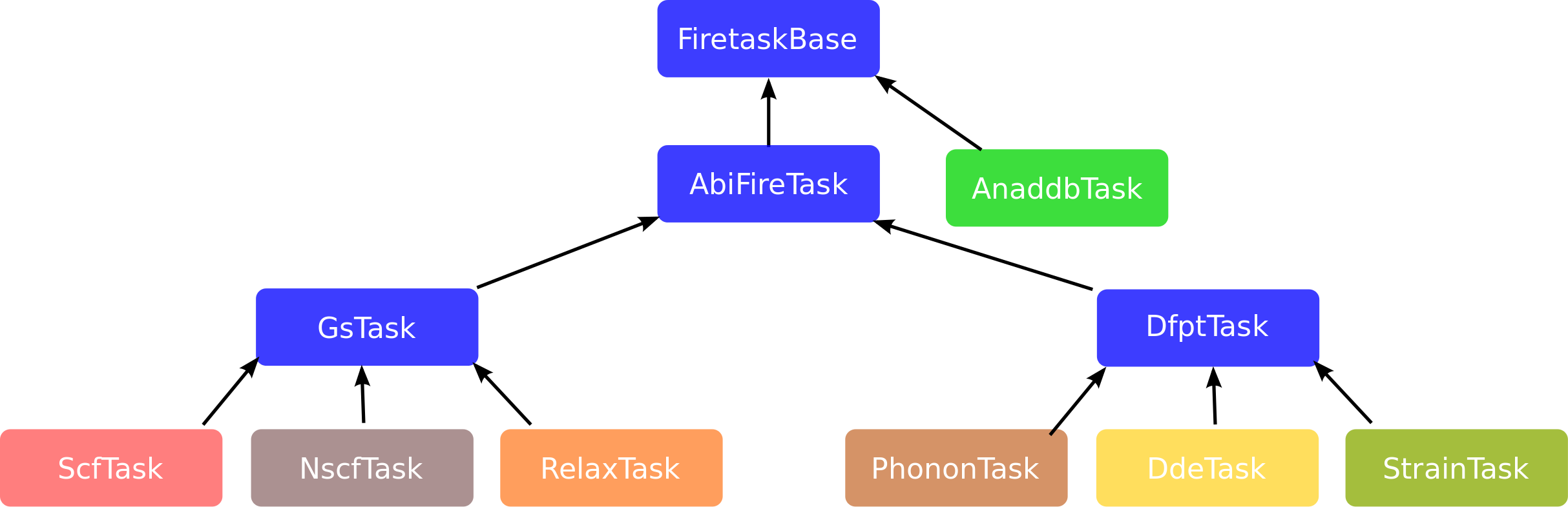
Object-oriented API and inheritance diagram
- Task objects to handle different types of calculations
- Automated handling of dependencies (WFK, DEN, DDB, …)
Workflow generators for common cases
- Relaxation
- Band structures
- Phonons
Templates for database insertion based on mongoengine and mongodb documents
How to build an AbiPy workflow
Let's start with an empty flow in the hello_flow directory
from abipy import flowtk
hello_flow = flowtk.Flow(workdir="hello_flow")
and use the graphviz tool after each step to show what's happening.
hello_flow.get_graphviz()
We also need a function returning two inputs for SCF/NSCF run:
def make_scf_nscf_inputs():
    """
    Build and return two input files for the GS-SCF and the GS-NSCF tasks.
    """
    multi = abilab.MultiDataset(structure="si.cif", pseudos="14si.pspnc", ndtset=2)

    # Set global variables (dataset1 and dataset2)
    multi.set_vars(ecut=6, nband=8)

    # Dataset 1 (GS-SCF run)
    multi[0].set_kmesh(ngkpt=[8, 8, 8], shiftk=[0, 0, 0])
    multi[0].set_vars(tolvrs=1e-6)

    # Dataset 2 (GS-NSCF run on a k-path)
    kptbounds = [
        [0.5, 0.0, 0.0], # L point
        [0.0, 0.0, 0.0], # Gamma point
        [0.0, 0.5, 0.5], # X point
    ]

    multi[1].set_kpath(ndivsm=6, kptbounds=kptbounds)
    multi[1].set_vars(tolwfr=1e-12)

    # Return two input files for the GS and the NSCF run
    scf_input, nscf_input = multi.split_datasets()
    return scf_input, nscf_input
In terms of factory functions, similar results can be obtained with:
from abipy.abio.factories import ebands_input
scf_input, nscf_input = ebands_input(structure="si.cif", pseudos="14si.pspnc")
To add a Task we create an AbinitInput and we register it in the flow:
scf_input, nscf_input = make_scf_nscf_inputs()

hello_flow.register_scf_task(scf_input, append=True)
hello_flow.get_graphviz()
To select the first work:
hello_flow[0]
To select the first task of the first work:
hello_flow[0][0]
How to define dependencies
- Let's add NSCF calculation that depends on the scf_task through the DEN file.
- Dependencies are specified via the {task: "file_ext"} dictionary
hello_flow.register_nscf_task(nscf_input, deps={hello_flow[0][0]: "DEN"},
                              append=True)

hello_flow.get_graphviz(engine="dot")
A Work is a list of Tasks and we can iterate with the syntax:
for task in hello_flow[0]:
    print(task)
Tasks can be connected to external files:
flow_with_file = flowtk.Flow(workdir="flow_with_file")

den_filepath = abidata.ref_file("si_DEN.nc")
flow_with_file.register_nscf_task(nscf_input, deps={den_filepath: "DEN"})

for nband in [10, 20]:
    flow_with_file.register_nscf_task(nscf_input.new_with_vars(nband=nband),
                                      deps={den_filepath: "DEN"}, append=False)

print("nband in tasks:", [task.input["nband"] for task in flow_with_file.iflat_tasks()])

flow_with_file.get_graphviz()
Phonon band structure of AlAs
Now we are finally ready for the calculation of the vibrational spectrum of AlAs.
Once we have a function returning an input for SCF calculations, it's just a matter of of passing the SCF input to the from_scf_input factory function
def build_flow_alas_phonons():
    """
    Build and return a Flow to compute the dynamical matrix on a (2, 2, 2) qmesh
    as well as DDK and Born effective charges.
    The final DDB with all perturbations will be merged automatically and placed
    in the Flow `outdir` directory.
    """
    from abipy import flowtk
    scf_input = make_scf_input(ecut=6, ngkpt=(4, 4, 4))
    return flowtk.PhononFlow.from_scf_input("flow_alas_phonons", scf_input,
                                            ph_ngqpt=(2, 2, 2), with_becs=True)
Abipy will call Abinit to get the list of DFPT perturbations and…
flow_phbands = build_flow_alas_phonons()
flow_phbands.get_graphviz()
To execute the flow, use the abirun.py script:
abirun.py flow_workdir scheduler
For futher info, see this notebook
DFPT workflows with Abiflows, Fireworks and MongoDB
- Databases makes life easier if one has to handle many calculations
Databases can be used to
- start calculations from previous results
- save the intermediate status of the jobs
- store the final results
Building an Abiflows workflow for DFPT requires:
from pseudo_dojo.core.pseudos import OfficialDojoTable
from abiflows.fireworks.workflows.abinit_workflows import PhononFullFWWorkflow

# Pseudopotential table from the PseudoDojo package
pseudo_table = OfficialDojoTable.from_dojodir('ONCVPSP-PBEsol-PDv0.4','standard')

# Create fireworks workflow with default settings
structure = abilab.Structure.from_file("si.cif")
wf = PhononFullFWWorkflow.from_factory(structure=structure, pseudos=pseudo_table)
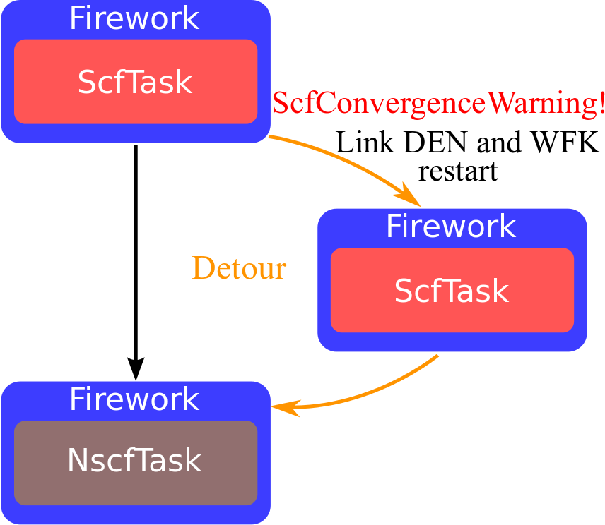
The dependency graph is similar to the ligthweigh version discussed before:
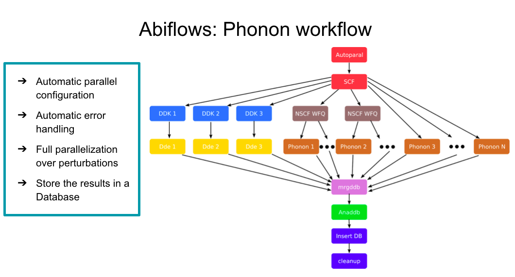
but now one can take advantage of MongoDb to run many calculations in a full automatic way:
from abiflows.fireworks.workflows.abinit_workflows import *
from abiflows.database.mongoengine.utils import DatabaseData
from abiflows.database.mongoengine.abinit_results import RelaxResult
from pseudo_dojo.core.pseudos import OfficialDojoTable

# Pseudopotential Table from PseudoDojo
pseudo_table = OfficialDojoTable.from_dojodir('ONCVPSP-PBEsol-PDv0.4','standard')

# Database with relaxed structures
source_db = DatabaseData(host='database_address', port=27017,
                         collection='collection_name_used_for_relax',
                         database='database_used_to_store_relax_calc')

# Database used to store DFPT results.
db = DatabaseData(host='database_address', port=27017, collection='phonon_bs',
                  database='database_name_eg_phonons')

# Connect to the database
source_db.connect_mongoengine()

# Download relaxed structure from the database.
with source_db.switch_collection(RelaxResult) as RelaxResult:
    relaxed_structure = RelaxResult.objects(mp_id="mp-149")[0].structure

wf = PhononFullFWWorkflow.from_factory(structure=structure, pseudos=pseudo_table)

wf.add_mongoengine_db_insertion(db)
wf.add_final_cleanup(["WFK", "1WF", "WFQ", "1POT", "1DEN"])
wf.add_to_db()
How to recostruct AbiPy objects from a MondoDb database
from abiflows.database.mongoengine.abinit_results import PhononResult

# Find results for SiC
r = PhononResult.objects(mp_id='mp-8062')[0]

# Get DDB object from the database.
with r.abinit_output.ddb.abiopen() as ddb:

    # Run anaddb
    phbst, phdos = ddb.anaget_phbst_and_phdos_files(ngqpt=[8, 8, 5])

    # Use AbiPy API
    phbst.phbands.plot_with_phdos(phdos.phdos, units='cm-1')
Conclusion
The ab-initio community is migrating to python to implement:
- Pre-processing and post-processing tools
- Web-based technologies to analyze/visualize data (e.g. jupyter notebooks …)
- High-level logic for scientific workflows and high-throughput applications
Difficulties for users:
- Installation of big software stack (C, C++, Fortran, Python, Javascript …)
- Multiple technologies under the hood (databases, JSON, HDF5, MPI/OMP …)
- Users are supposed to be familiar with programming techniques
Advantages for users:
- Traditional GUIs are still useful but researchers sometimes need programmatic interfaces to analyze raw data
- Several python packages to boost productivity and do better science
"An investment in knowledge pays the best interest" (B. Franklin)